Page 144 - Applied Statistics with R

144 CHAPTER 8. INFERENCE FOR SIMPLE LINEAR REGRESSION

stopping distance is between 2.8179187 and 5.0468988 feet, which is the interval
for .
1
Note that this 99% confidence interval does not contain the hypothesized value
of 0. Since it does not contain 0, it is equivalent to rejecting the test of ∶
0
= 0 vs ∶ ≠ 0 at = 0.01, which we had seen previously.
1
1
1
You should be somewhat suspicious of the confidence interval for , as it covers
0
negative values, which correspond to negative stopping distances. Technically
the interpretation would be that we are 99% confident that the average stopping
distance of a car traveling 0 miles per hour is between -35.7066103 and 0.5484205
feet, but we don’t really believe that, since we are actually certain that it would
be non-negative.
Note, we can extract specific values from this output a number of ways. This
code is not run, and instead, you should check how it relates to the output of
the code above.

confint(stop_dist_model, level = 0.99)[1,]
confint(stop_dist_model, level = 0.99)[1, 1]
confint(stop_dist_model, level = 0.99)[1, 2]
confint(stop_dist_model, parm = "(Intercept)", level = 0.99)
confint(stop_dist_model, level = 0.99)[2,]
confint(stop_dist_model, level = 0.99)[2, 1]
confint(stop_dist_model, level = 0.99)[2, 2]
confint(stop_dist_model, parm = "speed", level = 0.99)

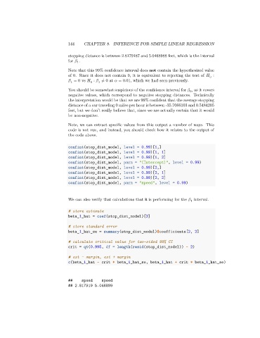
We can also verify that calculations that R is performing for the interval.
1
# store estimate
beta_1_hat = coef(stop_dist_model)[2]

# store standard error
beta_1_hat_se = summary(stop_dist_model)$coefficients[2, 2]

# calculate critical value for two-sided 99% CI
crit = qt(0.995, df = length(resid(stop_dist_model)) - 2)

# est - margin, est + margin
c(beta_1_hat - crit * beta_1_hat_se, beta_1_hat + crit * beta_1_hat_se)

## speed speed
## 2.817919 5.046899