Page 143 - Applied Statistics with R

8.6. CARS EXAMPLE 143

9
8

y 7

6

5

4
-1.0 -0.5 0.0 0.5 1.0

x

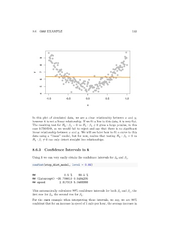
In this plot of simulated data, we see a clear relationship between and ,
however it is not a linear relationship. If we fit a line to this data, it is very flat.
The resulting test for ∶ = 0 vs ∶ ≠ 0 gives a large p-value, in this
1
0
1
1
case 0.7564548, so we would fail to reject and say that there is no significant
linear relationship between and . We will see later how to fit a curve to this
data using a “linear” model, but for now, realize that testing ∶ = 0 vs
1
0
∶ ≠ 0 can only detect straight line relationships.
1
1
8.6.3 Confidence Intervals in R
Using R we can very easily obtain the confidence intervals for and .
0
1
confint(stop_dist_model, level = 0.99)

## 0.5 % 99.5 %
## (Intercept) -35.706610 0.5484205
## speed 2.817919 5.0468988

This automatically calculates 99% confidence intervals for both and , the
0
1
first row for , the second row for .
1
0
For the cars example when interpreting these intervals, we say, we are 99%
confident that for an increase in speed of 1 mile per hour, the average increase in