Page 147 - Applied Statistics with R

8.9. CONFIDENCE AND PREDICTION BANDS 147

1 ( − ̄ ) 2
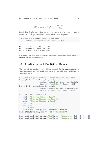
̂ ( ) ± /2, −2 ⋅ √1 + + .

To calculate this for a set of points in R notice there is only a minor change in
syntax from finding a confidence interval for the mean response.
predict(stop_dist_model, newdata = new_speeds,
interval = c("prediction"), level = 0.99)

## fit lwr upr
## 1 2.082949 -41.16099 45.32689
## 2 65.001489 22.87494 107.12803

Also notice that these two intervals are wider than the corresponding confidence
intervals for the mean response.

8.9 Confidence and Prediction Bands

Often we will like to plot both confidence intervals for the mean response and
prediction intervals for all possible values of . We calls these confidence and
prediction bands.

speed_grid = seq(min(cars$speed), max(cars$speed), by = 0.01)
dist_ci_band = predict(stop_dist_model,
newdata = data.frame(speed = speed_grid),
interval = "confidence", level = 0.99)
dist_pi_band = predict(stop_dist_model,
newdata = data.frame(speed = speed_grid),
interval = "prediction", level = 0.99)

plot(dist ~ speed, data = cars,
xlab = "Speed (in Miles Per Hour)",
ylab = "Stopping Distance (in Feet)",
main = "Stopping Distance vs Speed",
pch = 20,
cex = 2,
col = "grey",
ylim = c(min(dist_pi_band), max(dist_pi_band)))
abline(stop_dist_model, lwd = 5, col = "darkorange")

lines(speed_grid, dist_ci_band[,"lwr"], col = "dodgerblue", lwd = 3, lty = 2)
lines(speed_grid, dist_ci_band[,"upr"], col = "dodgerblue", lwd = 3, lty = 2)