Page 146 - Applied Statistics with R

146 CHAPTER 8. INFERENCE FOR SIMPLE LINEAR REGRESSION

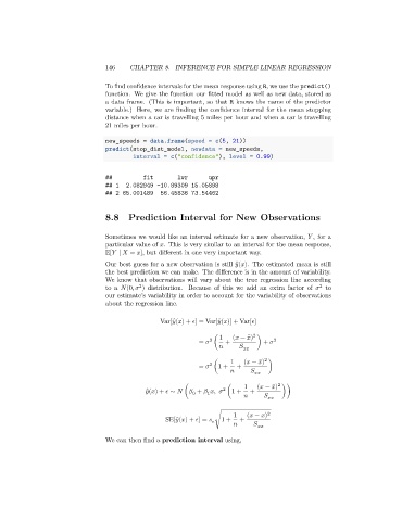
To find confidence intervals for the mean response using R, we use the predict()
function. We give the function our fitted model as well as new data, stored as
a data frame. (This is important, so that R knows the name of the predictor
variable.) Here, we are finding the confidence interval for the mean stopping
distance when a car is travelling 5 miles per hour and when a car is travelling
21 miles per hour.

new_speeds = data.frame(speed = c(5, 21))
predict(stop_dist_model, newdata = new_speeds,
interval = c("confidence"), level = 0.99)

## fit lwr upr
## 1 2.082949 -10.89309 15.05898
## 2 65.001489 56.45836 73.54462

8.8 Prediction Interval for New Observations

Sometimes we would like an interval estimate for a new observation, , for a
particular value of . This is very similar to an interval for the mean response,
E[ ∣ = ], but different in one very important way.

Our best guess for a new observation is still ̂( ). The estimated mean is still
the best prediction we can make. The difference is in the amount of variability.
We know that observations will vary about the true regression line according
2
2
to a (0, ) distribution. Because of this we add an extra factor of to
our estimate’s variability in order to account for the variability of observations
about the regression line.

Var[ ̂( ) + ] = Var[ ̂( )] + Var[ ]
1 ( − ̄ ) 2
2
= ( + ) + 2

1 ( − ̄ ) 2
2
= (1 + + )

1 ( − ̄ ) 2
2
̂ ( ) + ∼ ( + , (1 + + ))
1
0
1 ( − ̄ ) 2
SE[ ̂( ) + ] = √1 + +

We can then find a prediction interval using,