Page 150 - Applied Statistics with R

150 CHAPTER 8. INFERENCE FOR SIMPLE LINEAR REGRESSION

We can use the statistic to perform this test.

2

∑ ( ̂ − ̄) /1

= =1

2
∑ ( − ̂ ) /( − 2)
=1
In particular, we will reject the null when the statistic is large, that is, when
there is a low probability that the observations could have come from the null
model by chance. We will let R calculate the p-value for us.
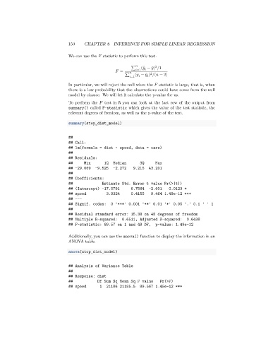
To perform the test in R you can look at the last row of the output from
summary() called F-statistic which gives the value of the test statistic, the
relevant degrees of freedom, as well as the p-value of the test.
summary(stop_dist_model)

##
## Call:
## lm(formula = dist ~ speed, data = cars)
##
## Residuals:
## Min 1Q Median 3Q Max
## -29.069 -9.525 -2.272 9.215 43.201
##
## Coefficients:
## Estimate Std. Error t value Pr(>|t|)
## (Intercept) -17.5791 6.7584 -2.601 0.0123 *
## speed 3.9324 0.4155 9.464 1.49e-12 ***
## ---
## Signif. codes: 0 '***' 0.001 '**' 0.01 '*' 0.05 '.' 0.1 ' ' 1
##
## Residual standard error: 15.38 on 48 degrees of freedom
## Multiple R-squared: 0.6511, Adjusted R-squared: 0.6438
## F-statistic: 89.57 on 1 and 48 DF, p-value: 1.49e-12

Additionally, you can use the anova() function to display the information in an
ANOVA table.

anova(stop_dist_model)

## Analysis of Variance Table
##
## Response: dist
## Df Sum Sq Mean Sq F value Pr(>F)
## speed 1 21186 21185.5 89.567 1.49e-12 ***