Page 178 - Applied Statistics with R

178 CHAPTER 9. MULTIPLE LINEAR REGRESSION

beta_0 = 5
beta_1 = -2
beta_2 = 6
sigma = 4

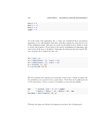
As is the norm with regression, the values are considered fixed and known
quantities, so we will simulate those first, and they remain the same for the rest
of the simulation study. Also note we create an x0 which is all 1, which we need
to create our X matrix. If you look at the matrix formulation of regression, this
unit vector of all 1s is a “predictor” that puts the intercept into the model. We
also calculate the C matrix for later use.

x0 = rep(1, n)
x1 = sample(seq(1, 10, length = n))
x2 = sample(seq(1, 10, length = n))
X = cbind(x0, x1, x2)
C = solve(t(X) %*% X)

We then simulate the response according the model above. Lastly, we place the
two predictors and response into a data frame. Note that we do not place x0
in the data frame. This is a result of R adding an intercept by default.

eps = rnorm(n, mean = 0, sd = sigma)
y = beta_0 + beta_1 * x1 + beta_2 * x2 + eps
sim_data = data.frame(x1, x2, y)

Plotting this data and fitting the regression produces the following plot.