Page 176 - Applied Statistics with R

176 CHAPTER 9. MULTIPLE LINEAR REGRESSION

Note that these are nested models, as the null model contains a subset of the
predictors from the full model, and no additional predictors. Both models have
an intercept as well as a coefficient in front of each of the predictors. We
0
could then write the null hypothesis for comparing these two models as,

∶ cyl = disp = hp = acc = 0
0
The alternative is simply that at least one of the from the null is not 0.

To perform this test in R we first define both models, then give them to the
anova() commands.

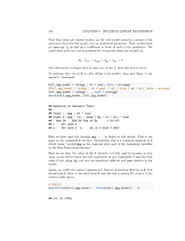
null_mpg_model = lm(mpg ~ wt + year, data = autompg)
#full_mpg_model = lm(mpg ~ wt + year + cyl + disp + hp + acc, data = autompg)
full_mpg_model = lm(mpg ~ ., data = autompg)
anova(null_mpg_model, full_mpg_model)

## Analysis of Variance Table
##
## Model 1: mpg ~ wt + year
## Model 2: mpg ~ cyl + disp + hp + wt + acc + year
## Res.Df RSS Df Sum of Sq F Pr(>F)
## 1 387 4556.6
## 2 383 4530.5 4 26.18 0.5533 0.6967

Here we have used the formula mpg ~ . to define to full model. This is the
same as the commented out line. Specifically, this is a common shortcut in R
which reads, “model mpg as the response with each of the remaining variables
in the data frame as predictors.”
Here we see that the value of the statistic is 0.553, and the p-value is very
large, so we fail to reject the null hypothesis at any reasonable and say that
none of cyl, disp, hp, and acc are significant with wt and year already in the
model.
Again, we verify the sums of squares and degrees of freedom directly in R. You
should match these to the table from R, and use this to match R’s output to the
written table above.

# SSDiff
sum((fitted(full_mpg_model) - fitted(null_mpg_model)) ^ 2)

## [1] 26.17981