Page 173 - Applied Statistics with R

9.3. SIGNIFICANCE OF REGRESSION 173

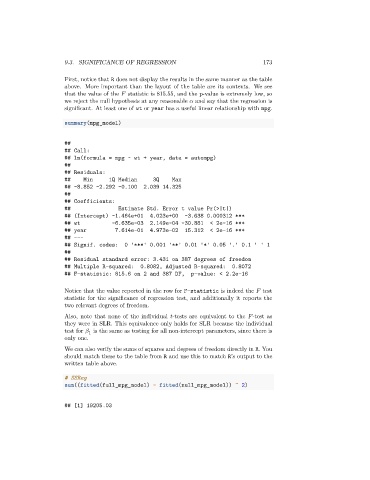
First, notice that R does not display the results in the same manner as the table
above. More important than the layout of the table are its contents. We see
that the value of the statistic is 815.55, and the p-value is extremely low, so
we reject the null hypothesis at any reasonable and say that the regression is
significant. At least one of wt or year has a useful linear relationship with mpg.

summary(mpg_model)

##
## Call:
## lm(formula = mpg ~ wt + year, data = autompg)
##
## Residuals:
## Min 1Q Median 3Q Max
## -8.852 -2.292 -0.100 2.039 14.325
##
## Coefficients:
## Estimate Std. Error t value Pr(>|t|)
## (Intercept) -1.464e+01 4.023e+00 -3.638 0.000312 ***
## wt -6.635e-03 2.149e-04 -30.881 < 2e-16 ***
## year 7.614e-01 4.973e-02 15.312 < 2e-16 ***
## ---
## Signif. codes: 0 '***' 0.001 '**' 0.01 '*' 0.05 '.' 0.1 ' ' 1
##
## Residual standard error: 3.431 on 387 degrees of freedom
## Multiple R-squared: 0.8082, Adjusted R-squared: 0.8072
## F-statistic: 815.6 on 2 and 387 DF, p-value: < 2.2e-16

Notice that the value reported in the row for F-statistic is indeed the test
statistic for the significance of regression test, and additionally it reports the
two relevant degrees of freedom.

Also, note that none of the individual -tests are equivalent to the -test as
they were in SLR. This equivalence only holds for SLR because the individual
test for is the same as testing for all non-intercept parameters, since there is
1
only one.
We can also verify the sums of squares and degrees of freedom directly in R. You
should match these to the table from R and use this to match R’s output to the
written table above.

# SSReg
sum((fitted(full_mpg_model) - fitted(null_mpg_model)) ^ 2)

## [1] 19205.03