Page 181 - Applied Statistics with R

9.5. SIMULATION 181

C[3, 3]

## [1] 0.00145343

C[2 + 1, 2 + 1]

## [1] 0.00145343

sigma ^ 2 * C[2 + 1, 2 + 1]

## [1] 0.02325487

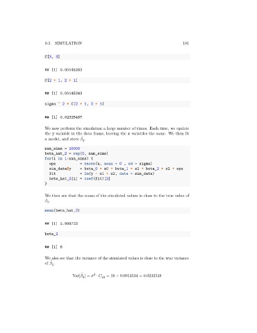
We now perform the simulation a large number of times. Each time, we update
the y variable in the data frame, leaving the x variables the same. We then fit
̂
a model, and store .
2
num_sims = 10000
beta_hat_2 = rep(0, num_sims)
for(i in 1:num_sims) {
eps = rnorm(n, mean = 0 , sd = sigma)
sim_data$y = beta_0 * x0 + beta_1 * x1 + beta_2 * x2 + eps
fit = lm(y ~ x1 + x2, data = sim_data)
beta_hat_2[i] = coef(fit)[3]
}

We then see that the mean of the simulated values is close to the true value of
.
2
mean(beta_hat_2)

## [1] 5.999723

beta_2

## [1] 6

We also see that the variance of the simulated values is close to the true variance
̂
of .
2
̂
2
Var[ ] = ⋅ 22 = 16 × 0.0014534 = 0.0232549
2