Page 198 - Applied Statistics with R

198 CHAPTER 11. CATEGORICAL PREDICTORS AND INTERACTIONS

Automatic
Manual
30

25
mpg
20

15

10
50 100 150 200 250 300

hp

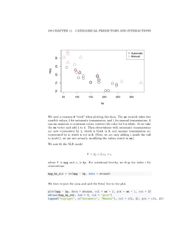
We used a common R “trick” when plotting this data. The am variable takes two
possible values; 0 for automatic transmission, and 1 for manual transmissions. R
can use numbers to represent colors, however the color for 0 is white. So we take
the am vector and add 1 to it. Then observations with automatic transmissions
are now represented by 1, which is black in R, and manual transmission are
represented by 2, which is red in R. (Note, we are only adding 1 inside the call
to plot(), we are not actually modifying the values stored in am.)

We now fit the SLR model

= + + ,
0
1 1
where is mpg and is hp. For notational brevity, we drop the index for
1
observations.

mpg_hp_slr = lm(mpg ~ hp, data = mtcars)

We then re-plot the data and add the fitted line to the plot.

plot(mpg ~ hp, data = mtcars, col = am + 1, pch = am + 1, cex = 2)
abline(mpg_hp_slr, lwd = 3, col = "grey")
legend("topright", c("Automatic", "Manual"), col = c(1, 2), pch = c(1, 2))