Page 201 - Applied Statistics with R

11.1. DUMMY VARIABLES 201

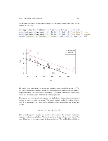
Re-plotting the data, we use these slopes and intercepts to add the “two” fitted
models to the plot.

plot(mpg ~ hp, data = mtcars, col = am + 1, pch = am + 1, cex = 2)
abline(int_auto, slope_auto, col = 1, lty = 1, lwd = 2) # add line for auto
abline(int_manu, slope_manu, col = 2, lty = 2, lwd = 2) # add line for manual
legend("topright", c("Automatic", "Manual"), col = c(1, 2), pch = c(1, 2))

Automatic
Manual
30

25
mpg
20

15

10
50 100 150 200 250 300

hp

We notice right away that the points are no longer systematically incorrect. The
red, manual observations vary about the red line in no particular pattern without
underestimating the observations as before. The black, automatic points vary
about the black line, also without an obvious pattern.
They say a picture is worth a thousand words, but as a statistician, sometimes a
picture is worth an entire analysis. The above picture makes it plainly obvious
that is significant, but let’s verify mathematically. Essentially we would like
2
to test:

∶ = 0 vs ∶ ≠ 0.
1
2
2
0
This is nothing new. Again, the math is the same as the multiple regression
analyses we have seen before. We could perform either a or test here. The
only difference is a slight change in interpretation. We could think of this as