Page 203 - Applied Statistics with R

11.2. INTERACTIONS 203

we see is the average change in for an increase in , no matter the value
1
1
of . Also, is always the difference in the average of for any value of .
2
2
1
These are two restrictions we won’t always want, so we need a way to specify a
more flexible model.
Here we restricted ourselves to a single numerical predictor and one dummy
1
variable . However, the concept of a dummy variable can be used with larger
2
multiple regression models. We only use a single numerical predictor here for
ease of visualization since we can think of the “two lines” interpretation. But
in general, we can think of a dummy variable as creating “two models,” one for
each category of a binary categorical variable.
11.2 Interactions

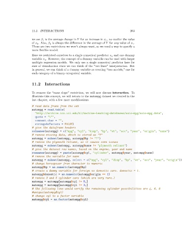
To remove the “same slope” restriction, we will now discuss interaction. To
illustrate this concept, we will return to the autompg dataset we created in the
last chapter, with a few more modifications.

# read data frame from the web
autompg = read.table(
"http://archive.ics.uci.edu/ml/machine-learning-databases/auto-mpg/auto-mpg.data",
quote = "\"",
comment.char = "",
stringsAsFactors = FALSE)
# give the dataframe headers
colnames(autompg) = c("mpg", "cyl", "disp", "hp", "wt", "acc", "year", "origin", "name")
# remove missing data, which is stored as "?"
autompg = subset(autompg, autompg$hp != "?")
# remove the plymouth reliant, as it causes some issues
autompg = subset(autompg, autompg$name != "plymouth reliant")
# give the dataset row names, based on the engine, year and name
rownames(autompg) = paste(autompg$cyl, "cylinder", autompg$year, autompg$name)
# remove the variable for name
autompg = subset(autompg, select = c("mpg", "cyl", "disp", "hp", "wt", "acc", "year", "origin"))
# change horsepower from character to numeric
autompg$hp = as.numeric(autompg$hp)
# create a dummy variable for foreign vs domestic cars. domestic = 1.
autompg$domestic = as.numeric(autompg$origin == 1)
# remove 3 and 5 cylinder cars (which are very rare.)
autompg = autompg[autompg$cyl != 5,]
autompg = autompg[autompg$cyl != 3,]
# the following line would verify the remaining cylinder possibilities are 4, 6, 8
#unique(autompg$cyl)
# change cyl to a factor variable
autompg$cyl = as.factor(autompg$cyl)