Page 227 - Applied Statistics with R

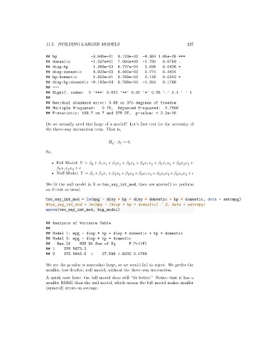
11.5. BUILDING LARGER MODELS 227

## hp -3.545e-01 8.123e-02 -4.364 1.65e-05 ***
## domestic -1.257e+01 7.064e+00 -1.780 0.0759 .
## disp:hp 1.369e-03 6.727e-04 2.035 0.0426 *
## disp:domestic 4.933e-02 6.400e-02 0.771 0.4414
## hp:domestic 1.852e-01 8.709e-02 2.126 0.0342 *
## disp:hp:domestic -9.163e-04 6.768e-04 -1.354 0.1766
## ---
## Signif. codes: 0 '***' 0.001 '**' 0.01 '*' 0.05 '.' 0.1 ' ' 1
##
## Residual standard error: 3.88 on 375 degrees of freedom
## Multiple R-squared: 0.76, Adjusted R-squared: 0.7556
## F-statistic: 169.7 on 7 and 375 DF, p-value: < 2.2e-16

Do we actually need this large of a model? Let’s first test for the necessity of
the three-way interaction term. That is,

∶ = 0.
0
7
So,

• Full Model: = + + + + + + +
5 1 3
1 1
6 2 3
3 3
4 1 2
0
2 2
+
7 1 2 3
• Null Model: = + + + + + + +
1 1
0
5 1 3
3 3
6 2 3
4 1 2
2 2
We fit the null model in R as two_way_int_mod, then use anova() to perform
an -test as usual.
two_way_int_mod = lm(mpg ~ disp * hp + disp * domestic + hp * domestic, data = autompg)
#two_way_int_mod = lm(mpg ~ (disp + hp + domestic) ^ 2, data = autompg)
anova(two_way_int_mod, big_model)
## Analysis of Variance Table
##
## Model 1: mpg ~ disp * hp + disp * domestic + hp * domestic
## Model 2: mpg ~ disp * hp * domestic
## Res.Df RSS Df Sum of Sq F Pr(>F)
## 1 376 5673.2
## 2 375 5645.6 1 27.599 1.8332 0.1766
We see the p-value is somewhat large, so we would fail to reject. We prefer the
smaller, less flexible, null model, without the three-way interaction.
A quick note here: the full model does still “fit better.” Notice that it has a
smaller RMSE than the null model, which means the full model makes smaller
(squared) errors on average.