Page 222 - Applied Statistics with R

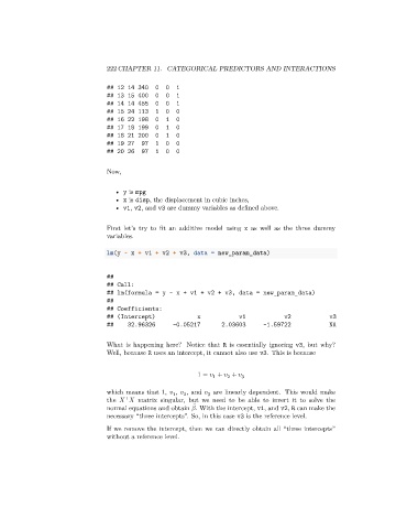
222 CHAPTER 11. CATEGORICAL PREDICTORS AND INTERACTIONS

## 12 14 340 0 0 1
## 13 15 400 0 0 1
## 14 14 455 0 0 1
## 15 24 113 1 0 0
## 16 22 198 0 1 0
## 17 18 199 0 1 0
## 18 21 200 0 1 0
## 19 27 97 1 0 0
## 20 26 97 1 0 0

Now,

• y is mpg
• x is disp, the displacement in cubic inches,
• v1, v2, and v3 are dummy variables as defined above.

First let’s try to fit an additive model using x as well as the three dummy
variables.

lm(y ~ x + v1 + v2 + v3, data = new_param_data)

##
## Call:
## lm(formula = y ~ x + v1 + v2 + v3, data = new_param_data)
##
## Coefficients:
## (Intercept) x v1 v2 v3
## 32.96326 -0.05217 2.03603 -1.59722 NA

What is happening here? Notice that R is essentially ignoring v3, but why?
Well, because R uses an intercept, it cannot also use v3. This is because

1 = + + 3
2
1
which means that 1, , , and are linearly dependent. This would make
1
2
3
⊤
the matrix singular, but we need to be able to invert it to solve the
̂
normal equations and obtain . With the intercept, v1, and v2, R can make the
necessary “three intercepts”. So, in this case v3 is the reference level.
If we remove the intercept, then we can directly obtain all “three intercepts”
without a reference level.