Page 256 - Applied Statistics with R

256 CHAPTER 12. ANALYSIS OF VARIANCE

The row for Factor B tests:

∶ All = 0. vs ∶ Not all are 0.
0
1

• Null Model: = + + . (Only Factor A Model.)

• Alternative Model: = + + + . (Additive Model.)

We reject the null when the statistic is large. Under the null hypothesis,
the distribution of the test statistic is with degrees of freedom − 1 and
( − 1).
The row for Factor A tests:

∶ All = 0. vs ∶ Not all are 0.

0
1
• Null Model: = + + . (Only Factor B Model.)

• Alternative Model: = + + + . (Additive Model.)

We reject the null when the statistic is large. Under the null hypothesis, the
distribution of the test statistic is with degrees of freedom −1 and ( −1).
These tests should be performed according to the model hierarchy. First con-
sider the test of interaction. If it is significant, we select the interaction model
and perform no further testing. If interaction is not significant, we then consider
the necessity of the individual factors of the additive model.

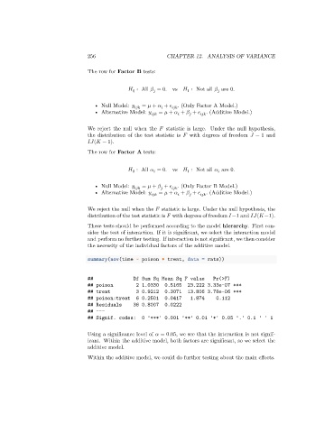
summary(aov(time ~ poison * treat, data = rats))

## Df Sum Sq Mean Sq F value Pr(>F)
## poison 2 1.0330 0.5165 23.222 3.33e-07 ***
## treat 3 0.9212 0.3071 13.806 3.78e-06 ***
## poison:treat 6 0.2501 0.0417 1.874 0.112
## Residuals 36 0.8007 0.0222
## ---
## Signif. codes: 0 '***' 0.001 '**' 0.01 '*' 0.05 '.' 0.1 ' ' 1

Using a significance level of = 0.05, we see that the interaction is not signif-
icant. Within the additive model, both factors are significant, so we select the
additive model.
Within the additive model, we could do further testing about the main effects.