Page 258 - Applied Statistics with R

258 CHAPTER 12. ANALYSIS OF VARIANCE

TukeyHSD(aov(time ~ poison + treat, data = rats))

## Tukey multiple comparisons of means
## 95% family-wise confidence level
##
## Fit: aov(formula = time ~ poison + treat, data = rats)
##
## $poison
## diff lwr upr p adj
## II-I -0.073125 -0.2089936 0.0627436 0.3989657
## III-I -0.341250 -0.4771186 -0.2053814 0.0000008
## III-II -0.268125 -0.4039936 -0.1322564 0.0000606
##
## $treat
## diff lwr upr p adj
## B-A 0.36250000 0.18976135 0.53523865 0.0000083
## C-A 0.07833333 -0.09440532 0.25107198 0.6221729
## D-A 0.22000000 0.04726135 0.39273865 0.0076661
## C-B -0.28416667 -0.45690532 -0.11142802 0.0004090
## D-B -0.14250000 -0.31523865 0.03023865 0.1380432
## D-C 0.14166667 -0.03107198 0.31440532 0.1416151

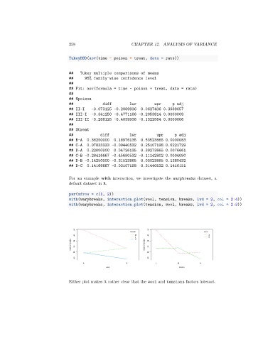
For an example with interaction, we investigate the warpbreaks dataset, a
default dataset in R.

par(mfrow = c(1, 2))
with(warpbreaks, interaction.plot(wool, tension, breaks, lwd = 2, col = 2:4))
with(warpbreaks, interaction.plot(tension, wool, breaks, lwd = 2, col = 2:3))

45 45
tension wool
40 M 40 A
L H 35 B
mean of breaks 30 mean of breaks 30
35
25 25
20 20
A B L M H
wool tension

Either plot makes it rather clear that the wool and tensions factors interact.