Page 254 - Applied Statistics with R

254 CHAPTER 12. ANALYSIS OF VARIANCE

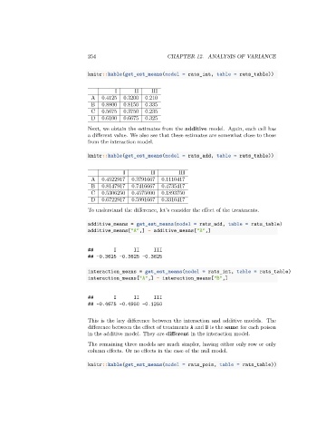
knitr::kable(get_est_means(model = rats_int, table = rats_table))

I II III
A 0.4125 0.3200 0.210
B 0.8800 0.8150 0.335
C 0.5675 0.3750 0.235
D 0.6100 0.6675 0.325

Next, we obtain the estimates from the additive model. Again, each cell has
a different value. We also see that these estimates are somewhat close to those
from the interaction model.

knitr::kable(get_est_means(model = rats_add, table = rats_table))

I II III
A 0.4522917 0.3791667 0.1110417
B 0.8147917 0.7416667 0.4735417
C 0.5306250 0.4575000 0.1893750
D 0.6722917 0.5991667 0.3310417
To understand the difference, let’s consider the effect of the treatments.

additive_means = get_est_means(model = rats_add, table = rats_table)
additive_means["A",] - additive_means["B",]

## I II III
## -0.3625 -0.3625 -0.3625

interaction_means = get_est_means(model = rats_int, table = rats_table)
interaction_means["A",] - interaction_means["B",]

## I II III
## -0.4675 -0.4950 -0.1250

This is the key difference between the interaction and additive models. The
difference between the effect of treatments A and B is the same for each poison
in the additive model. They are different in the interaction model.

The remaining three models are much simpler, having either only row or only
column effects. Or no effects in the case of the null model.

knitr::kable(get_est_means(model = rats_pois, table = rats_table))