Page 252 - Applied Statistics with R

252 CHAPTER 12. ANALYSIS OF VARIANCE

levels(rats$treat)

## [1] "A" "B" "C" "D"

Here, 48 rats were randomly assigned both one of three poisons and one of four
possible treatments. The experimenters then measures their survival time in
tens of hours. A total of 12 groups, each with 4 replicates.
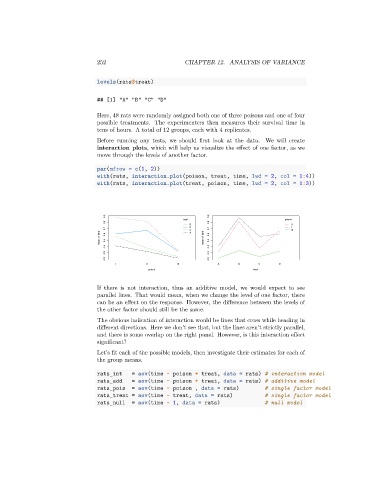
Before running any tests, we should first look at the data. We will create
interaction plots, which will help us visualize the effect of one factor, as we
move through the levels of another factor.

par(mfrow = c(1, 2))
with(rats, interaction.plot(poison, treat, time, lwd = 2, col = 1:4))
with(rats, interaction.plot(treat, poison, time, lwd = 2, col = 1:3))

0.9 0.9
treat poison
0.8 0.8
B II
0.7 D C A 0.7 I III
mean of time 0.6 0.5 mean of time 0.6 0.5
0.4 0.4
0.3 0.3
0.2 0.2
I II III A B C D
poison treat

If there is not interaction, thus an additive model, we would expect to see
parallel lines. That would mean, when we change the level of one factor, there
can be an effect on the response. However, the difference between the levels of
the other factor should still be the same.
The obvious indication of interaction would be lines that cross while heading in
different directions. Here we don’t see that, but the lines aren’t strictly parallel,
and there is some overlap on the right panel. However, is this interaction effect
significant?
Let’s fit each of the possible models, then investigate their estimates for each of
the group means.
rats_int = aov(time ~ poison * treat, data = rats) # interaction model
rats_add = aov(time ~ poison + treat, data = rats) # additive model
rats_pois = aov(time ~ poison , data = rats) # single factor model
rats_treat = aov(time ~ treat, data = rats) # single factor model
rats_null = aov(time ~ 1, data = rats) # null model