Page 255 - Applied Statistics with R

12.5. TWO-WAY ANOVA 255

I II III
A 0.6175 0.544375 0.27625
B 0.6175 0.544375 0.27625
C 0.6175 0.544375 0.27625
D 0.6175 0.544375 0.27625

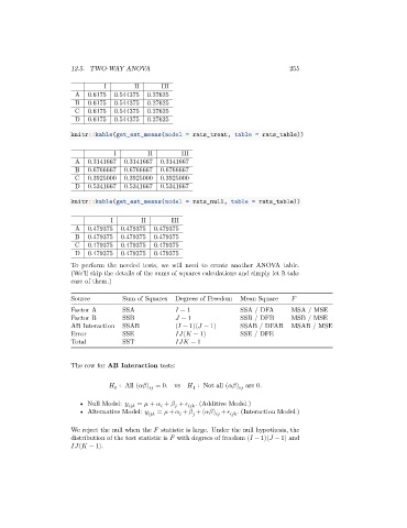
knitr::kable(get_est_means(model = rats_treat, table = rats_table))

I II III
A 0.3141667 0.3141667 0.3141667
B 0.6766667 0.6766667 0.6766667
C 0.3925000 0.3925000 0.3925000
D 0.5341667 0.5341667 0.5341667

knitr::kable(get_est_means(model = rats_null, table = rats_table))

I II III
A 0.479375 0.479375 0.479375
B 0.479375 0.479375 0.479375
C 0.479375 0.479375 0.479375
D 0.479375 0.479375 0.479375
To perform the needed tests, we will need to create another ANOVA table.
(We’ll skip the details of the sums of squares calculations and simply let R take
care of them.)

Source Sum of Squares Degrees of Freedom Mean Square

Factor A SSA − 1 SSA / DFA MSA / MSE
Factor B SSB − 1 SSB / DFB MSB / MSE
AB Interaction SSAB ( − 1)( − 1) SSAB / DFAB MSAB / MSE
Error SSE ( − 1) SSE / DFE
Total SST − 1

The row for AB Interaction tests:

∶ All ( ) = 0. vs ∶ Not all ( ) are 0.

0

1
• Null Model: = + + + . (Additive Model.)

• Alternative Model: = + + +( ) + . (Interaction Model.)

We reject the null when the statistic is large. Under the null hypothesis, the
distribution of the test statistic is with degrees of freedom ( − 1)( − 1) and
( − 1).