Page 299 - Applied Statistics with R

13.4. DATA ANALYSIS EXAMPLES 299

## $ cyl : Factor w/ 3 levels "4","6","8": 3 3 3 3 3 3 3 3 3 3 ...
## $ disp : num 307 350 318 304 302 429 454 440 455 390 ...
## $ hp : num 130 165 150 150 140 198 220 215 225 190 ...
## $ wt : num 3504 3693 3436 3433 3449 ...
## $ acc : num 12 11.5 11 12 10.5 10 9 8.5 10 8.5 ...
## $ year : int 70 70 70 70 70 70 70 70 70 70 ...
## $ origin : int 1 1 1 1 1 1 1 1 1 1 ...
## $ domestic: num 1 1 1 1 1 1 1 1 1 1 ...

big_model = lm(mpg ~ disp * hp * domestic, data = autompg)

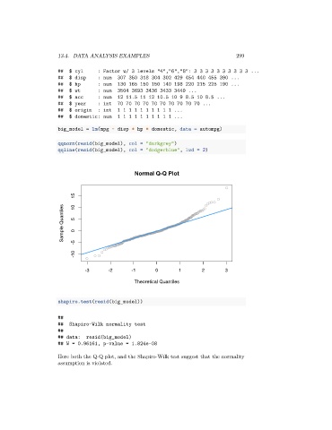
qqnorm(resid(big_model), col = "darkgrey")
qqline(resid(big_model), col = "dodgerblue", lwd = 2)

Normal Q-Q Plot

15 10

Sample Quantiles 5 0

-5

-10

-3 -2 -1 0 1 2 3
Theoretical Quantiles

shapiro.test(resid(big_model))

##
## Shapiro-Wilk normality test
##
## data: resid(big_model)
## W = 0.96161, p-value = 1.824e-08

Here both the Q-Q plot, and the Shapiro-Wilk test suggest that the normality
assumption is violated.