Page 305 - Applied Statistics with R

14.1. RESPONSE TRANSFORMATION 305

## Signif. codes: 0 '***' 0.001 '**' 0.01 '*' 0.05 '.' 0.1 ' ' 1
##
## Residual standard error: 27360 on 98 degrees of freedom
## Multiple R-squared: 0.8341, Adjusted R-squared: 0.8324
## F-statistic: 492.8 on 1 and 98 DF, p-value: < 2.2e-16

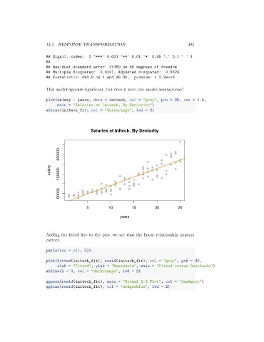
This model appears significant, but does it meet the model assumptions?

plot(salary ~ years, data = initech, col = "grey", pch = 20, cex = 1.5,
main = "Salaries at Initech, By Seniority")
abline(initech_fit, col = "darkorange", lwd = 2)

Salaries at Initech, By Seniority

250000

salary 150000

50000

5 10 15 20 25
years

Adding the fitted line to the plot, we see that the linear relationship appears
correct.

par(mfrow = c(1, 2))

plot(fitted(initech_fit), resid(initech_fit), col = "grey", pch = 20,
xlab = "Fitted", ylab = "Residuals", main = "Fitted versus Residuals")
abline(h = 0, col = "darkorange", lwd = 2)

qqnorm(resid(initech_fit), main = "Normal Q-Q Plot", col = "darkgrey")
qqline(resid(initech_fit), col = "dodgerblue", lwd = 2)