Page 310 - Applied Statistics with R

310 CHAPTER 14. TRANSFORMATIONS

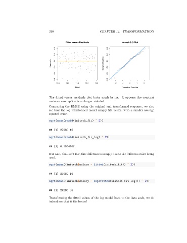
Fitted versus Residuals Normal Q-Q Plot
0.4 0.4

0.2 0.2
Residuals 0.0 -0.2 Sample Quantiles 0.0 -0.2

-0.4 -0.4

-0.6 -0.6
10.5 11.0 11.5 12.0 12.5 -2 -1 0 1 2
Fitted Theoretical Quantiles

The fitted versus residuals plot looks much better. It appears the constant
variance assumption is no longer violated.
Comparing the RMSE using the original and transformed response, we also
see that the log transformed model simply fits better, with a smaller average
squared error.
sqrt(mean(resid(initech_fit) ^ 2))

## [1] 27080.16

sqrt(mean(resid(initech_fit_log) ^ 2))

## [1] 0.1934907

But wait, that isn’t fair, this difference is simply due to the different scales being
used.
sqrt(mean((initech$salary - fitted(initech_fit)) ^ 2))

## [1] 27080.16

sqrt(mean((initech$salary - exp(fitted(initech_fit_log))) ^ 2))

## [1] 24280.36

Transforming the fitted values of the log model back to the data scale, we do
indeed see that it fits better!