Page 338 - Applied Statistics with R

338 CHAPTER 14. TRANSFORMATIONS

##
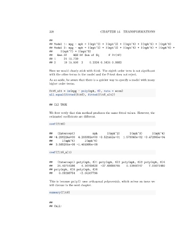
## Model 1: mpg ~ mph + I(mph^2) + I(mph^3) + I(mph^4) + I(mph^5) + I(mph^6)
## Model 2: mpg ~ mph + I(mph^2) + I(mph^3) + I(mph^4) + I(mph^5) + I(mph^6) +
## I(mph^7) + I(mph^8)
## Res.Df RSS Df Sum of Sq F Pr(>F)
## 1 21 15.739
## 2 19 15.506 2 0.2324 0.1424 0.8682

Here we would clearly stick with fit6. The eighth order term is not significant
with the other terms in the model and the F-test does not reject.
As an aside, be aware that there is a quicker way to specify a model with many
higher order terms.

fit6_alt = lm(mpg ~ poly(mph, 6), data = econ)
all.equal(fitted(fit6), fitted(fit6_alt))

## [1] TRUE

We first verify that this method produces the same fitted values. However, the
estimated coefficients are different.

coef(fit6)

## (Intercept) mph I(mph^2) I(mph^3) I(mph^4)
## -4.206224e+00 4.203382e+00 -3.521452e-01 1.579340e-02 -3.472665e-04
## I(mph^5) I(mph^6)
## 3.585201e-06 -1.401995e-08

coef(fit6_alt)

## (Intercept) poly(mph, 6)1 poly(mph, 6)2 poly(mph, 6)3 poly(mph, 6)4
## 24.40714286 4.16769628 -27.66685755 0.13446747 7.01671480
## poly(mph, 6)5 poly(mph, 6)6
## 0.09288754 -2.04307796

This is because poly() uses orthogonal polynomials, which solves an issue we
will discuss in the next chapter.

summary(fit6)

##
## Call: