Page 340 - Applied Statistics with R

340 CHAPTER 14. TRANSFORMATIONS

## Residual standard error: 0.8657 on 21 degrees of freedom
## Multiple R-squared: 0.9815, Adjusted R-squared: 0.9762
## F-statistic: 186 on 6 and 21 DF, p-value: < 2.2e-16

Notice though that the p-value for testing the degree 6 term is the same. Because
of this, for the most part we can use these interchangeably.

To use poly() to obtain the same results as using I() repeatedly, we would
need to set raw = TRUE.

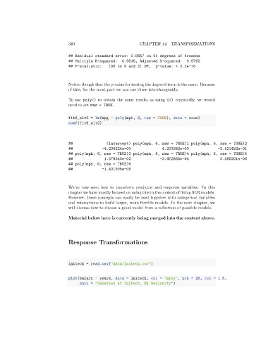
fit6_alt2 = lm(mpg ~ poly(mph, 6, raw = TRUE), data = econ)
coef(fit6_alt2)

## (Intercept) poly(mph, 6, raw = TRUE)1 poly(mph, 6, raw = TRUE)2
## -4.206224e+00 4.203382e+00 -3.521452e-01
## poly(mph, 6, raw = TRUE)3 poly(mph, 6, raw = TRUE)4 poly(mph, 6, raw = TRUE)5
## 1.579340e-02 -3.472665e-04 3.585201e-06
## poly(mph, 6, raw = TRUE)6
## -1.401995e-08

We’ve now seen how to transform predictor and response variables. In this
chapter we have mostly focused on using this in the context of fixing SLR models.
However, these concepts can easily be used together with categorical variables
and interactions to build larger, more flexible models. In the next chapter, we
will discuss how to choose a good model from a collection of possible models.

Material below here is currently being merged into the content above.

Response Transformations

initech = read.csv("data/initech.csv")

plot(salary ~ years, data = initech, col = "grey", pch = 20, cex = 1.5,
main = "Salaries at Initech, By Seniority")