Page 335 - Applied Statistics with R

14.2. PREDICTOR TRANSFORMATION 335

##
## Residual standard error: 0.8657 on 21 degrees of freedom
## Multiple R-squared: 0.9815, Adjusted R-squared: 0.9762
## F-statistic: 186 on 6 and 21 DF, p-value: < 2.2e-16

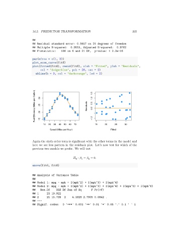
par(mfrow = c(1, 2))
plot_econ_curve(fit6)
plot(fitted(fit6), resid(fit6), xlab = "Fitted", ylab = "Residuals",
col = "dodgerblue", pch = 20, cex = 2)
abline(h = 0, col = "darkorange", lwd = 2)

Fuel Efficiency (Miles per Gallon) 30 25 20 Residuals 1.5 1.0 0.5 0.0

15
10 20 30 40 50 60 70 -1.0 15 20 25 30

Speed (Miles per Hour) Fitted

Again the sixth order term is significant with the other terms in the model and
here we see less pattern in the residuals plot. Let’s now test for which of the
previous two models we prefer. We will test

∶ = = 0.
5
6
0
anova(fit4, fit6)

## Analysis of Variance Table
##
## Model 1: mpg ~ mph + I(mph^2) + I(mph^3) + I(mph^4)
## Model 2: mpg ~ mph + I(mph^2) + I(mph^3) + I(mph^4) + I(mph^5) + I(mph^6)
## Res.Df RSS Df Sum of Sq F Pr(>F)
## 1 23 19.922
## 2 21 15.739 2 4.1828 2.7905 0.0842 .
## ---
## Signif. codes: 0 '***' 0.001 '**' 0.01 '*' 0.05 '.' 0.1 ' ' 1