Page 333 - Applied Statistics with R

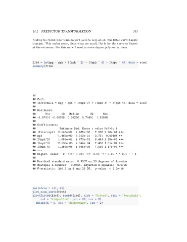
14.2. PREDICTOR TRANSFORMATION 333

Adding the third order term doesn’t seem to help at all. The fitted curve hardly
changes. This makes sense, since what we would like is for the curve to flatten
at the extremes. For this we will need an even degree polynomial term.

fit4 = lm(mpg ~ mph + I(mph ^ 2) + I(mph ^ 3) + I(mph ^ 4), data = econ)
summary(fit4)

##
## Call:
## lm(formula = mpg ~ mph + I(mph^2) + I(mph^3) + I(mph^4), data = econ)
##
## Residuals:
## Min 1Q Median 3Q Max
## -1.57410 -0.60308 0.04236 0.74481 1.93038
##
## Coefficients:
## Estimate Std. Error t value Pr(>|t|)
## (Intercept) 2.146e+01 2.965e+00 7.238 2.28e-07 ***
## mph -1.468e+00 3.913e-01 -3.751 0.00104 **
## I(mph^2) 1.081e-01 1.673e-02 6.463 1.35e-06 ***
## I(mph^3) -2.130e-03 2.844e-04 -7.488 1.31e-07 ***
## I(mph^4) 1.255e-05 1.665e-06 7.539 1.17e-07 ***
## ---
## Signif. codes: 0 '***' 0.001 '**' 0.01 '*' 0.05 '.' 0.1 ' ' 1
##
## Residual standard error: 0.9307 on 23 degrees of freedom
## Multiple R-squared: 0.9766, Adjusted R-squared: 0.9726
## F-statistic: 240.2 on 4 and 23 DF, p-value: < 2.2e-16

par(mfrow = c(1, 2))
plot_econ_curve(fit4)
plot(fitted(fit4), resid(fit4), xlab = "Fitted", ylab = "Residuals",
col = "dodgerblue", pch = 20, cex = 2)
abline(h = 0, col = "darkorange", lwd = 2)