Page 334 - Applied Statistics with R

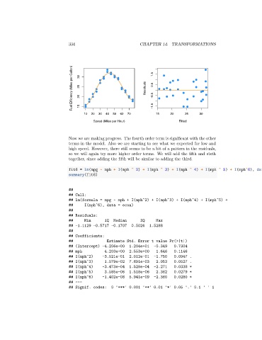
334 CHAPTER 14. TRANSFORMATIONS

Fuel Efficiency (Miles per Gallon) 30 25 20 Residuals 1.5 0.5 -0.5

15

10 20 30 40 50 60 70 -1.5 15 20 25 30
Speed (Miles per Hour) Fitted

Now we are making progress. The fourth order term is significant with the other
terms in the model. Also we are starting to see what we expected for low and
high speed. However, there still seems to be a bit of a pattern in the residuals,
so we will again try more higher order terms. We will add the fifth and sixth
together, since adding the fifth will be similar to adding the third.

fit6 = lm(mpg ~ mph + I(mph ^ 2) + I(mph ^ 3) + I(mph ^ 4) + I(mph ^ 5) + I(mph^6), data = econ)
summary(fit6)

##
## Call:
## lm(formula = mpg ~ mph + I(mph^2) + I(mph^3) + I(mph^4) + I(mph^5) +
## I(mph^6), data = econ)
##
## Residuals:
## Min 1Q Median 3Q Max
## -1.1129 -0.5717 -0.1707 0.5026 1.5288
##
## Coefficients:
## Estimate Std. Error t value Pr(>|t|)
## (Intercept) -4.206e+00 1.204e+01 -0.349 0.7304
## mph 4.203e+00 2.553e+00 1.646 0.1146
## I(mph^2) -3.521e-01 2.012e-01 -1.750 0.0947 .
## I(mph^3) 1.579e-02 7.691e-03 2.053 0.0527 .
## I(mph^4) -3.473e-04 1.529e-04 -2.271 0.0338 *
## I(mph^5) 3.585e-06 1.518e-06 2.362 0.0279 *
## I(mph^6) -1.402e-08 5.941e-09 -2.360 0.0280 *
## ---
## Signif. codes: 0 '***' 0.001 '**' 0.01 '*' 0.05 '.' 0.1 ' ' 1