Page 380 - Applied Statistics with R

380 CHAPTER 15. COLLINEARITY

sd(beta_hat_bad[, 1])

## [1] 1.633294

sd(beta_hat_good[, 1])

## [1] 0.5484684

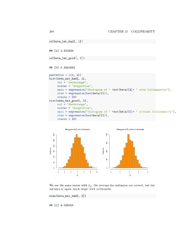
par(mfrow = c(1, 2))
hist(beta_hat_bad[, 2],
col = "darkorange",
border = "dodgerblue",
main = expression("Histogram of " *hat(beta)[2]* " with Collinearity"),
xlab = expression(hat(beta)[2]),
breaks = 20)
hist(beta_hat_good[, 2],
col = "darkorange",
border = "dodgerblue",
main = expression("Histogram of " *hat(beta)[2]* " without Collinearity"),
xlab = expression(hat(beta)[2]),
breaks = 20)

^
^
Histogram of β 2 with Collinearity Histogram of β 2 without Collinearity
300 400
250
300
200
Frequency 150 Frequency 200

100
100
50
0 0
-2 0 2 4 6 8 10 2 3 4 5 6
^ ^
β 2 β 2

We see the same issues with . On average the estimates are correct, but the
2
variance is again much larger with collinearity.
mean(beta_hat_bad[, 2])

## [1] 4.025059