Page 381 - Applied Statistics with R

15.3. SIMULATION 381

mean(beta_hat_good[, 2])

## [1] 4.004913

sd(beta_hat_bad[, 2])

## [1] 1.642592

sd(beta_hat_good[, 2])

## [1] 0.5470381

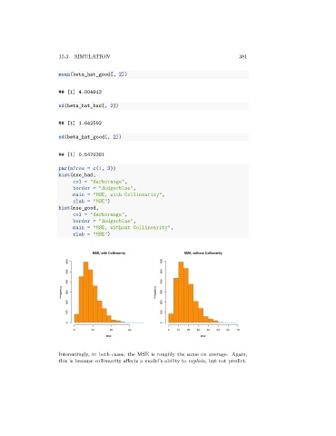
par(mfrow = c(1, 2))
hist(mse_bad,
col = "darkorange",
border = "dodgerblue",
main = "MSE, with Collinearity",
xlab = "MSE")
hist(mse_good,
col = "darkorange",
border = "dodgerblue",
main = "MSE, without Collinearity",
xlab = "MSE")

MSE, with Collinearity MSE, without Collinearity
600 600
500 500

400 400
Frequency 300 Frequency 300

200 200
100 100

0 0
0 20 40 60 0 10 20 30 40 50 60 70
MSE MSE

Interestingly, in both cases, the MSE is roughly the same on average. Again,
this is because collinearity affects a model’s ability to explain, but not predict.