Page 379 - Applied Statistics with R

15.3. SIMULATION 379

par(mfrow = c(1, 2))
hist(beta_hat_bad[, 1],
col = "darkorange",
border = "dodgerblue",
main = expression("Histogram of " *hat(beta)[1]* " with Collinearity"),
xlab = expression(hat(beta)[1]),
breaks = 20)
hist(beta_hat_good[, 1],
col = "darkorange",
border = "dodgerblue",
main = expression("Histogram of " *hat(beta)[1]* " without Collinearity"),
xlab = expression(hat(beta)[1]),
breaks = 20)

^ ^
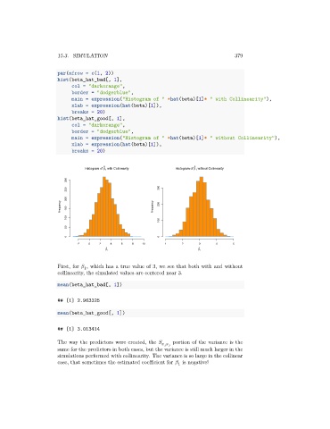
Histogram of β 1 with Collinearity Histogram of β 1 without Collinearity
300
250 300
200
Frequency 150 Frequency 200

100
100
50
0 0
-2 0 2 4 6 8 10 1 2 3 4 5
^ ^
β 1 β 1

First, for , which has a true value of 3, we see that both with and without
1
collinearity, the simulated values are centered near 3.
mean(beta_hat_bad[, 1])

## [1] 2.963325

mean(beta_hat_good[, 1])

## [1] 3.013414

The way the predictors were created, the portion of the variance is the

same for the predictors in both cases, but the variance is still much larger in the
simulations performed with collinearity. The variance is so large in the collinear
case, that sometimes the estimated coefficient for is negative!
1