Page 378 - Applied Statistics with R

378 CHAPTER 15. COLLINEARITY

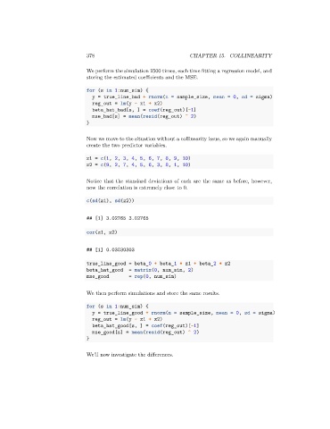
We perform the simulation 2500 times, each time fitting a regression model, and
storing the estimated coefficients and the MSE.

for (s in 1:num_sim) {
y = true_line_bad + rnorm(n = sample_size, mean = 0, sd = sigma)
reg_out = lm(y ~ x1 + x2)
beta_hat_bad[s, ] = coef(reg_out)[-1]
mse_bad[s] = mean(resid(reg_out) ^ 2)
}

Now we move to the situation without a collinearity issue, so we again manually
create the two predictor variables.

z1 = c(1, 2, 3, 4, 5, 6, 7, 8, 9, 10)
z2 = c(9, 2, 7, 4, 5, 6, 3, 8, 1, 10)

Notice that the standard deviations of each are the same as before, however,
now the correlation is extremely close to 0.

c(sd(z1), sd(z2))

## [1] 3.02765 3.02765

cor(z1, z2)

## [1] 0.03030303

true_line_good = beta_0 + beta_1 * z1 + beta_2 * z2
beta_hat_good = matrix(0, num_sim, 2)
mse_good = rep(0, num_sim)

We then perform simulations and store the same results.

for (s in 1:num_sim) {
y = true_line_good + rnorm(n = sample_size, mean = 0, sd = sigma)
reg_out = lm(y ~ z1 + z2)
beta_hat_good[s, ] = coef(reg_out)[-1]
mse_good[s] = mean(resid(reg_out) ^ 2)
}

We’ll now investigate the differences.