Page 377 - Applied Statistics with R

15.3. SIMULATION 377

15.3 Simulation

Here we simulate example data with and without collinearity. We will note the
difference in the distribution of the estimates of the parameters, in particular
their variance. However, we will also notice the similarity in their .
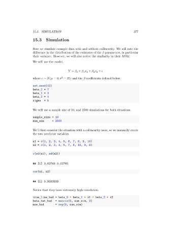
We will use the model,

= + + +
0
2 2
1 1
2
where ∼ ( = 0, = 25) and the coefficients defined below.
set.seed(42)
beta_0 = 7
beta_1 = 3
beta_2 = 4
sigma = 5

We will use a sample size of 10, and 2500 simulations for both situations.

sample_size = 10
num_sim = 2500

We’ll first consider the situation with a collinearity issue, so we manually create
the two predictor variables.

x1 = c(1, 2, 3, 4, 5, 6, 7, 8, 9, 10)
x2 = c(1, 2, 3, 4, 5, 7, 6, 10, 9, 8)

c(sd(x1), sd(x2))

## [1] 3.02765 3.02765

cor(x1, x2)

## [1] 0.9393939

Notice that they have extremely high correlation.

true_line_bad = beta_0 + beta_1 * x1 + beta_2 * x2
beta_hat_bad = matrix(0, num_sim, 2)
mse_bad = rep(0, num_sim)