Page 68 - Applied Statistics with R

68 CHAPTER 5. PROBABILITY AND STATISTICS IN R

2
For example, consider a random variable which is ( = 2, = 25). (Note,
2
we are parameterizing using the variance . R however uses the standard
deviation.)
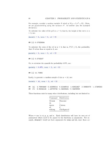
To calculate the value of the pdf at x = 3, that is, the height of the curve at x
= 3, use:

dnorm(x = 3, mean = 2, sd = 5)

## [1] 0.07820854

To calculate the value of the cdf at x = 3, that is, ( ≤ 3), the probability
that is less than or equal to 3, use:
pnorm(q = 3, mean = 2, sd = 5)

## [1] 0.5792597

Or, to calculate the quantile for probability 0.975, use:
qnorm(p = 0.975, mean = 2, sd = 5)

## [1] 11.79982

Lastly, to generate a random sample of size n = 10, use:

rnorm(n = 10, mean = 2, sd = 5)

## [1] 4.76864449 -3.43986614 8.43148012 1.40652427 3.56455078 1.17269243
## [7] 6.65026116 1.28709756 -1.04638281 -0.04809939

These functions exist for many other distributions, including but not limited to:

Command Distribution
*binom Binomial
*t t
*pois Poisson
*f F
*chisq Chi-Squared

Where * can be d, p, q, and r. Each distribution will have its own set of
parameters which need to be passed to the functions as arguments. For ex-
ample, dbinom() would not have arguments for mean and sd, since those are