Page 64 - Applied Statistics with R

64 CHAPTER 4. SUMMARIZING DATA

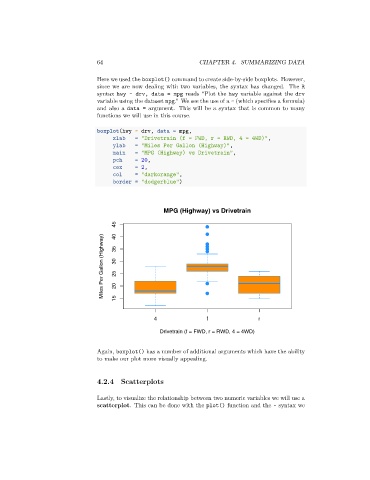
Here we used the boxplot() command to create side-by-side boxplots. However,
since we are now dealing with two variables, the syntax has changed. The R
syntax hwy ~ drv, data = mpg reads “Plot the hwy variable against the drv
variable using the dataset mpg.” We see the use of a ~ (which specifies a formula)
and also a data = argument. This will be a syntax that is common to many
functions we will use in this course.

boxplot(hwy ~ drv, data = mpg,
xlab = "Drivetrain (f = FWD, r = RWD, 4 = 4WD)",
ylab = "Miles Per Gallon (Highway)",
main = "MPG (Highway) vs Drivetrain",
pch = 20,
cex = 2,
col = "darkorange",
border = "dodgerblue")

MPG (Highway) vs Drivetrain

45 40
Miles Per Gallon (Highway) 35 30 25 20

15

4 f r

Drivetrain (f = FWD, r = RWD, 4 = 4WD)

Again, boxplot() has a number of additional arguments which have the ability
to make our plot more visually appealing.

4.2.4 Scatterplots

Lastly, to visualize the relationship between two numeric variables we will use a
scatterplot. This can be done with the plot() function and the ~ syntax we