Page 79 - Applied Statistics with R

5.3. SIMULATION 79

To estimate (0 < < 2) we will find the proportion of values of (among

4
the 10 values of generated) that are between 0 and 2.

mean(0 < differences & differences < 2)

## [1] 0.9222

2
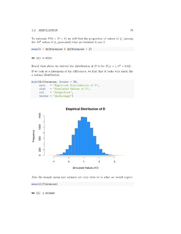
Recall that above we derived the distribution of to be ( = 1, = 0.32)
If we look at a histogram of the differences, we find that it looks very much like
a normal distribution.

hist(differences, breaks = 20,
main = "Empirical Distribution of D",
xlab = "Simulated Values of D",
col = "dodgerblue",
border = "darkorange")

Empirical Distribution of D
1400

1000

Frequency 600

200

0

-1 0 1 2 3
Simulated Values of D

Also the sample mean and variance are very close to to what we would expect.

mean(differences)

## [1] 1.001423