Page 98 - Applied Statistics with R

98 CHAPTER 7. SIMPLE LINEAR REGRESSION

+ ∑ = ∑
1
0

=1 =1

2
∑ + ∑ = ∑

1

0
=1 =1 =1
Finally, we finish solving the system of equations.

(∑ )(∑ )
∑ − =1 =1

̂
= =1 2 =
1
2
∑ − (∑ =1 )
=1
̂
̂

= ̄ − ̄
1
0
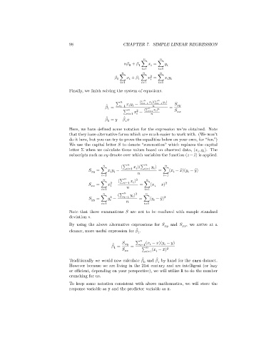
Here, we have defined some notation for the expression we’ve obtained. Note
that they have alternative forms which are much easier to work with. (We won’t
do it here, but you can try to prove the equalities below on your own, for “fun.”)
We use the capital letter to denote “summation” which replaces the capital
letter Σ when we calculate these values based on observed data, ( , ). The

subscripts such as denote over which variables the function ( − ̄) is applied.
(∑ )(∑ )
= ∑ − =1 =1 = ∑( − ̄ )( − ̄ )

=1 =1
(∑ ) 2
2
= ∑ − =1 = ∑( − ̄ ) 2

=1 =1
(∑ ) 2
2
= ∑ − =1 = ∑( − ̄) 2

=1 =1
Note that these summations are not to be confused with sample standard
deviation .
By using the above alternative expressions for and , we arrive at a

̂
cleaner, more useful expression for .
1

∑ ( − ̄ )( − ̄)
̂
= = =1
1
∑ =1 ( − ̄ ) 2

̂
̂
Traditionally we would now calculate and by hand for the cars dataset.
0
1
However because we are living in the 21st century and are intelligent (or lazy
or efficient, depending on your perspective), we will utilize R to do the number
crunching for us.
To keep some notation consistent with above mathematics, we will store the
response variable as y and the predictor variable as x.