Page 111 - Applied Statistics with R

7.4. THE LM FUNCTION 111

stop_dist_model$residuals

## 1 2 3 4 5 6 7
## 3.849460 11.849460 -5.947766 12.052234 2.119825 -7.812584 -3.744993
## 8 9 10 11 12 13 14
## 4.255007 12.255007 -8.677401 2.322599 -15.609810 -9.609810 -5.609810
## 15 16 17 18 19 20 21
## -1.609810 -7.542219 0.457781 0.457781 12.457781 -11.474628 -1.474628
## 22 23 24 25 26 27 28
## 22.525372 42.525372 -21.407036 -15.407036 12.592964 -13.339445 -5.339445
## 29 30 31 32 33 34 35
## -17.271854 -9.271854 0.728146 -11.204263 2.795737 22.795737 30.795737
## 36 37 38 39 40 41 42
## -21.136672 -11.136672 10.863328 -29.069080 -13.069080 -9.069080 -5.069080
## 43 44 45 46 47 48 49
## 2.930920 -2.933898 -18.866307 -6.798715 15.201285 16.201285 43.201285
## 50
## 4.268876

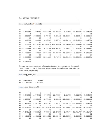
Another way to access stored information in stop_dist_model are the coef(),
resid(), and fitted() functions. These return the coefficients, residuals, and
fitted values, respectively.

coef(stop_dist_model)

## (Intercept) speed
## -17.579095 3.932409

resid(stop_dist_model)

## 1 2 3 4 5 6 7
## 3.849460 11.849460 -5.947766 12.052234 2.119825 -7.812584 -3.744993
## 8 9 10 11 12 13 14
## 4.255007 12.255007 -8.677401 2.322599 -15.609810 -9.609810 -5.609810
## 15 16 17 18 19 20 21
## -1.609810 -7.542219 0.457781 0.457781 12.457781 -11.474628 -1.474628
## 22 23 24 25 26 27 28
## 22.525372 42.525372 -21.407036 -15.407036 12.592964 -13.339445 -5.339445
## 29 30 31 32 33 34 35
## -17.271854 -9.271854 0.728146 -11.204263 2.795737 22.795737 30.795737
## 36 37 38 39 40 41 42
## -21.136672 -11.136672 10.863328 -29.069080 -13.069080 -9.069080 -5.069080
## 43 44 45 46 47 48 49