Page 110 - Applied Statistics with R

110 CHAPTER 7. SIMPLE LINEAR REGRESSION

cex = 2,
col = "grey")
abline(stop_dist_model, lwd = 3, col = "darkorange")

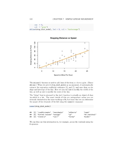
Stopping Distance vs Speed

120 100
Stopping Distance (in Feet) 80 60 40

0 20
5 10 15 20 25

Speed (in Miles Per Hour)

The abline() function is used to add lines of the form + to a plot. (Hence
abline.) When we give it stop_dist_model as an argument, it automatically
̂
̂
extracts the regression coefficient estimates ( and ) and uses them as the
0
1
slope and intercept of the line. Here we also use lwd to modify the width of the
line, as well as col to modify the color of the line.
The “thing” that is returned by the lm() function is actually an object of class
lm which is a list. The exact details of this are unimportant unless you are
seriously interested in the inner-workings of R, but know that we can determine
the names of the elements of the list using the names() command.

names(stop_dist_model)

## [1] "coefficients" "residuals" "effects" "rank"
## [5] "fitted.values" "assign" "qr" "df.residual"
## [9] "xlevels" "call" "terms" "model"

We can then use this information to, for example, access the residuals using the
$ operator.