Page 112 - Applied Statistics with R

112 CHAPTER 7. SIMPLE LINEAR REGRESSION

## 2.930920 -2.933898 -18.866307 -6.798715 15.201285 16.201285 43.201285
## 50
## 4.268876

fitted(stop_dist_model)

## 1 2 3 4 5 6 7 8
## -1.849460 -1.849460 9.947766 9.947766 13.880175 17.812584 21.744993 21.744993
## 9 10 11 12 13 14 15 16
## 21.744993 25.677401 25.677401 29.609810 29.609810 29.609810 29.609810 33.542219
## 17 18 19 20 21 22 23 24
## 33.542219 33.542219 33.542219 37.474628 37.474628 37.474628 37.474628 41.407036
## 25 26 27 28 29 30 31 32
## 41.407036 41.407036 45.339445 45.339445 49.271854 49.271854 49.271854 53.204263
## 33 34 35 36 37 38 39 40
## 53.204263 53.204263 53.204263 57.136672 57.136672 57.136672 61.069080 61.069080
## 41 42 43 44 45 46 47 48
## 61.069080 61.069080 61.069080 68.933898 72.866307 76.798715 76.798715 76.798715
## 49 50
## 76.798715 80.731124

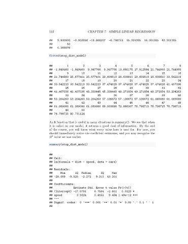
An R function that is useful in many situations is summary(). We see that when
it is called on our model, it returns a good deal of information. By the end
of the course, you will know what every value here is used for. For now, you
should immediately notice the coefficient estimates, and you may recognize the
2
value we saw earlier.
summary(stop_dist_model)

##
## Call:
## lm(formula = dist ~ speed, data = cars)
##
## Residuals:
## Min 1Q Median 3Q Max
## -29.069 -9.525 -2.272 9.215 43.201
##
## Coefficients:
## Estimate Std. Error t value Pr(>|t|)
## (Intercept) -17.5791 6.7584 -2.601 0.0123 *
## speed 3.9324 0.4155 9.464 1.49e-12 ***
## ---
## Signif. codes: 0 '***' 0.001 '**' 0.01 '*' 0.05 '.' 0.1 ' ' 1
##