Page 113 - Applied Statistics with R

7.4. THE LM FUNCTION 113

## Residual standard error: 15.38 on 48 degrees of freedom
## Multiple R-squared: 0.6511, Adjusted R-squared: 0.6438
## F-statistic: 89.57 on 1 and 48 DF, p-value: 1.49e-12

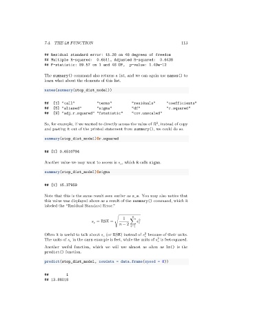
The summary() command also returns a list, and we can again use names() to
learn what about the elements of this list.
names(summary(stop_dist_model))

## [1] "call" "terms" "residuals" "coefficients"
## [5] "aliased" "sigma" "df" "r.squared"
## [9] "adj.r.squared" "fstatistic" "cov.unscaled"

2
So, for example, if we wanted to directly access the value of , instead of copy
and pasting it out of the printed statement from summary(), we could do so.

summary(stop_dist_model)$r.squared

## [1] 0.6510794

Another value we may want to access is , which R calls sigma.

summary(stop_dist_model)$sigma

## [1] 15.37959

Note that this is the same result seen earlier as s_e. You may also notice that
this value was displayed above as a result of the summary() command, which R
labeled the “Residual Standard Error.”

1
= RSE = √ ∑ 2

− 2
=1
2
Often it is useful to talk about (or RSE) instead of because of their units.

2
The units of in the cars example is feet, while the units of is feet-squared.

Another useful function, which we will use almost as often as lm() is the
predict() function.
predict(stop_dist_model, newdata = data.frame(speed = 8))
## 1
## 13.88018