Page 119 - Applied Statistics with R

7.6. SIMULATING SLR 119

x_vals = seq(from = 0, to = 10, length.out = num_obs)
# set.seed(1)
# x_vals = runif(num_obs, 0, 10)

We then generate the values according the specified functional relationship.

y_vals = beta_0 + beta_1 * x_vals + epsilon

The data, ( , ), represent a possible sample from the true distribution. Now

to check how well the method of least squares works, we use lm() to fit the
model to our simulated data, then take a look at the estimated coefficients.
sim_fit = lm(y_vals ~ x_vals)
coef(sim_fit)

## (Intercept) x_vals
## 4.832639 -1.831401

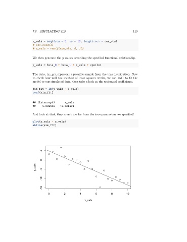
And look at that, they aren’t too far from the true parameters we specified!

plot(y_vals ~ x_vals)
abline(sim_fit)

5

0
y_vals -5

-10

-15

0 2 4 6 8 10
x_vals