Page 120 - Applied Statistics with R

120 CHAPTER 7. SIMPLE LINEAR REGRESSION

We should say here, that we’re being sort of lazy, and not the good kinda of
lazy that could be considered efficient. Any time you simulate data, you should
consider doing two things: writing a function, and storing the data in a data
frame.
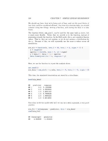
The function below, sim_slr(), can be used for the same task as above, but
is much more flexible. Notice that we provide x to the function, instead of
generating x inside the function. In the SLR model, the are considered known

values. That is, they are not random, so we do not assume a distribution for
the . Because of this, we will repeatedly use the same x values across all

simulations.

sim_slr = function(x, beta_0 = 10, beta_1 = 5, sigma = 1) {
n = length(x)
epsilon = rnorm(n, mean = 0, sd = sigma)
y = beta_0 + beta_1 * x + epsilon
data.frame(predictor = x, response = y)
}

Here, we use the function to repeat the analysis above.

set.seed(1)
sim_data = sim_slr(x = x_vals, beta_0 = 5, beta_1 = -2, sigma = 3)

This time, the simulated observations are stored in a data frame.

head(sim_data)

## predictor response
## 1 0.0 3.1206386
## 2 0.5 4.5509300
## 3 1.0 0.4931142
## 4 1.5 6.7858424
## 5 2.0 1.9885233
## 6 2.5 -2.4614052

Now when we fit the model with lm() we can use a data argument, a very good
practice.

sim_fit = lm(response ~ predictor, data = sim_data)
coef(sim_fit)

## (Intercept) predictor
## 4.832639 -1.831401