Page 117 - Applied Statistics with R

7.5. MAXIMUM LIKELIHOOD ESTIMATION (MLE) APPROACH 117

1
2
2
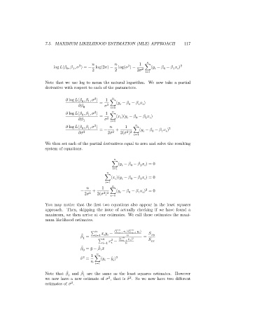
log ( , , ) = − log(2 ) − log( ) − ∑( − − ) 2
0
1
0

1
2 2 2 2
=1
Note that we use log to mean the natural logarithm. We now take a partial
derivative with respect to each of the parameters.

2
log ( , , ) = 1 ∑( − − )
1
0
0 2 =1 0 1

2
log ( , , ) = 1 ∑( )( − − )
1
0
1 2 =1 0 1
2
log ( , , ) 1 2
0
1
0

1
2 = − 2 2 + 2( ) ∑( − − )
2 2
=1
We then set each of the partial derivatives equal to zero and solve the resulting
system of equations.

∑( − − ) = 0
0
1

=1

∑( )( − − ) = 0
0

1

=1
1
2
− + ∑( − − ) = 0
1
0

2 2
2 2 2( )
=1
You may notice that the first two equations also appear in the least squares
approach. Then, skipping the issue of actually checking if we have found a
maximum, we then arrive at our estimates. We call these estimates the maxi-
mum likelihood estimates.

(∑ )(∑ )
∑ − =1 =1
̂
= =1 (∑ ) 2 =
1
2
∑ − =1
=1
̂
̂
= ̄ − ̄

0
1
1
2
̂ = ∑( − ̂ ) 2

=1
̂
̂
Note that and are the same as the least squares estimates. However
1
0
2
2
we now have a new estimate of , that is ̂ . So we now have two different
2
estimates of .