Page 125 - Applied Statistics with R

125

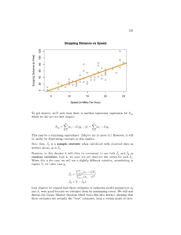
Stopping Distance vs Speed

120 100
Stopping Distance (in Feet) 80 60 40

0 20
5 10 15 20 25

Speed (in Miles Per Hour)

To get started, we’ll note that there is another equivalent expression for
which we did not see last chapter,

= ∑( − ̄ )( − ̄ ) = ∑( − ̄ ) .

=1 =1
This may be a surprising equivalence. (Maybe try to prove it.) However, it will
be useful for illustrating concepts in this chapter.
̂
Note that, is a sample statistic when calculated with observed data as
1
̂
written above, as is .
0
̂
̂
However, in this chapter it will often be convenient to use both and as
0
1
random variables, that is, we have not yet observed the values for each .

When this is the case, we will use a slightly different notation, substituting in
capital for lower case .

∑ ( − ̄ )

̂
= =1
1

∑ ( − ̄ ) 2
=1
̂
̂
̄
= − ̄
0
1
Last chapter we argued that these estimates of unknown model parameters 0
and were good because we obtained them by minimizing errors. We will now
1
discuss the Gauss–Markov theorem which takes this idea further, showing that
these estimates are actually the “best” estimates, from a certain point of view.