Page 126 - Applied Statistics with R

126 CHAPTER 8. INFERENCE FOR SIMPLE LINEAR REGRESSION

8.1 Gauss–Markov Theorem

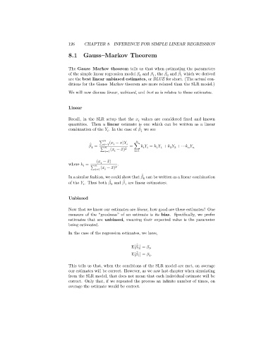
The Gauss–Markov theorem tells us that when estimating the parameters
̂
̂
of the simple linear regression model and , the and which we derived
1
0
1
0
are the best linear unbiased estimates, or BLUE for short. (The actual con-
ditions for the Gauss–Markov theorem are more relaxed than the SLR model.)
We will now discuss linear, unbiased, and best as is relates to these estimates.
Linear

Recall, in the SLR setup that the values are considered fixed and known

quantities. Then a linear estimate is one which can be written as a linear
̂
combination of the . In the case of we see
1

∑ ( − ̄ )
̂
= =1 = ∑ = + + ⋯

1
1 1

2 2
∑ ( − ̄ ) 2
=1 =1
( − ̄ )

where = .

∑ ( − ̄ ) 2
=1
̂
In a similar fashion, we could show that can be written as a linear combination
0
̂
̂
of the . Thus both and are linear estimators.

0
1
Unbiased
Now that we know our estimates are linear, how good are these estimates? One
measure of the “goodness” of an estimate is its bias. Specifically, we prefer
estimates that are unbiased, meaning their expected value is the parameter
being estimated.
In the case of the regression estimates, we have,
̂
E[ ] = 0
0
̂
E[ ] = .
1
1
This tells us that, when the conditions of the SLR model are met, on average
our estimates will be correct. However, as we saw last chapter when simulating
from the SLR model, that does not mean that each individual estimate will be
correct. Only that, if we repeated the process an infinite number of times, on
average the estimate would be correct.