Page 130 - Applied Statistics with R

130 CHAPTER 8. INFERENCE FOR SIMPLE LINEAR REGRESSION

̂
∼ (3, 0.04).
0
That is,

̂
E[ ] = 6
1
̂
Var[ ] = 0.1176238
1
and
̂
E[ ] = 3
0
̂
Var[ ] = 0.04.
0
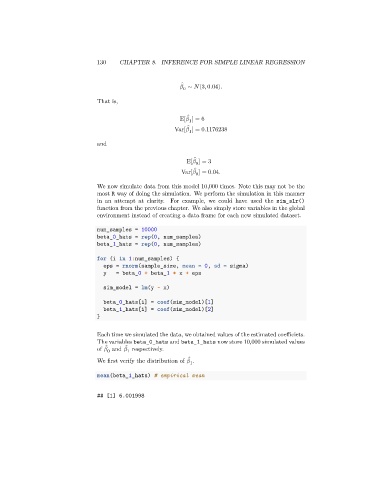
We now simulate data from this model 10,000 times. Note this may not be the
most R way of doing the simulation. We perform the simulation in this manner
in an attempt at clarity. For example, we could have used the sim_slr()
function from the previous chapter. We also simply store variables in the global
environment instead of creating a data frame for each new simulated dataset.

num_samples = 10000
beta_0_hats = rep(0, num_samples)
beta_1_hats = rep(0, num_samples)

for (i in 1:num_samples) {
eps = rnorm(sample_size, mean = 0, sd = sigma)
y = beta_0 + beta_1 * x + eps

sim_model = lm(y ~ x)

beta_0_hats[i] = coef(sim_model)[1]
beta_1_hats[i] = coef(sim_model)[2]
}

Each time we simulated the data, we obtained values of the estimated coefficiets.
The variables beta_0_hats and beta_1_hats now store 10,000 simulated values
̂
̂
of and respectively.
1
0
̂
We first verify the distribution of .
1
mean(beta_1_hats) # empirical mean
## [1] 6.001998