Page 129 - Applied Statistics with R

8.2. SAMPLING DISTRIBUTIONS 129

• = 6
1
2
• = 4
Then, based on the above, we should find that

2
̂
∼ ( , )
1
1
and

2
̄
̂
2
∼ ( , ( 1 + )) .
0
0

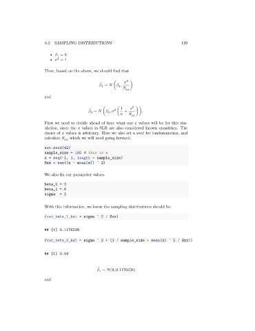
First we need to decide ahead of time what our values will be for this sim-
ulation, since the values in SLR are also considered known quantities. The
choice of values is arbitrary. Here we also set a seed for randomization, and
calculate which we will need going forward.
set.seed(42)
sample_size = 100 # this is n
x = seq(-1, 1, length = sample_size)
Sxx = sum((x - mean(x)) ^ 2)

We also fix our parameter values.
beta_0 = 3
beta_1 = 6
sigma = 2

With this information, we know the sampling distributions should be:

(var_beta_1_hat = sigma ^ 2 / Sxx)

## [1] 0.1176238

(var_beta_0_hat = sigma ^ 2 * (1 / sample_size + mean(x) ^ 2 / Sxx))

## [1] 0.04

̂
∼ (6, 0.1176238)
1
and