Page 128 - Applied Statistics with R

128 CHAPTER 8. INFERENCE FOR SIMPLE LINEAR REGRESSION

̂
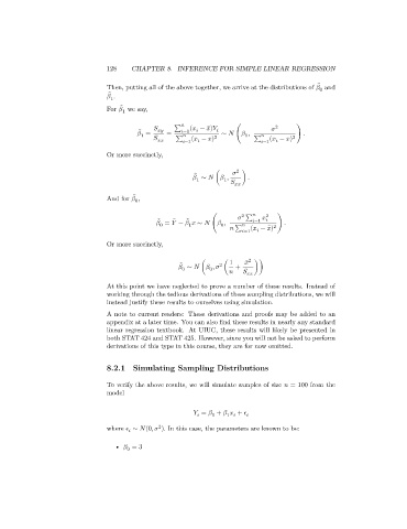
Then, putting all of the above together, we arrive at the distributions of and
0
̂
.
1
̂
For we say,
1

∑ ( − ̄ ) 2
̂

= = =1 ∼ ( , ) .

1
1
∑ =1 ( − ̄ ) 2 ∑ =1 ( − ̄ ) 2

Or more succinctly,
2
̂
∼ ( , ) .
1
1
̂
And for ,
0
2
∑ 2
̄
̂
̂
̄
= − ∼ ( , =1 ) .
0
1
0
∑ ( − ̄ ) 2
=1
Or more succinctly,
2
̄
̂
2
∼ ( , ( 1 + ))
0
0

At this point we have neglected to prove a number of these results. Instead of
working through the tedious derivations of these sampling distributions, we will
instead justify these results to ourselves using simulation.
A note to current readers: These derivations and proofs may be added to an
appendix at a later time. You can also find these results in nearly any standard
linear regression textbook. At UIUC, these results will likely be presented in
both STAT 424 and STAT 425. However, since you will not be asked to perform
derivations of this type in this course, they are for now omitted.
8.2.1 Simulating Sampling Distributions
To verify the above results, we will simulate samples of size = 100 from the
model
= + +

0
1
2
where ∼ (0, ). In this case, the parameters are known to be:

• = 3
0