Page 156 - Applied Statistics with R

156 CHAPTER 9. MULTIPLE LINEAR REGRESSION

with respect to , , and . How do we do so? It is another straightforward
0
1
2
multivariate calculus problem. All we have done is add an extra variable since
we did this last time. So again, we take a derivative with respect to each of
, , and and set them equal to zero, then solve the resulting system of
2
1
0
equations. That is,
= 0
0

= 0
1

= 0
2
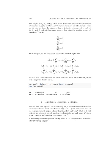
After doing so, we will once again obtain the normal equations.

+ ∑ + ∑ 2 = ∑
2
0
1
1
=1 =1 =1

2
∑ + ∑ + ∑ = ∑
1
1
1
1 2
2
0
1
=1 =1 =1 =1

∑ + ∑ + ∑ 2 2 = ∑
0
2
1 2
1
2
2
=1 =1 =1 =1
We now have three equations and three variables, which we could solve, or we
could simply let R solve for us.
mpg_model = lm(mpg ~ wt + year, data = autompg)
coef(mpg_model)
## (Intercept) wt year
## -14.637641945 -0.006634876 0.761401955
̂ = −14.6376419 + −0.0066349 + 0.761402 2
1
Here we have once again fit our model using lm(), however we have introduced
a new syntactical element. The formula mpg ~ wt + year now reads: “model
the response variable mpg as a linear function of wt and year”. That is, it will
estimate an intercept, as well as slope coefficients for wt and year. We then
extract these as we have done before using coef().

In the multiple linear regression setting, some of the interpretations of the co-
efficients change slightly.