Page 160 - Applied Statistics with R

160 CHAPTER 9. MULTIPLE LINEAR REGRESSION

1 1 ̂ 1
⎡ ⎤ ⎡ ⎤ ⎡ ̂ ⎤
= ⎢ 2 ⎥ = ⎢ 2 ⎥ − ⎢ 2 ⎥ .
⎢ ⋮ ⎥ ⎢ ⋮ ⎥ ⎢ ⋮ ⎥
⎣ ⎦ ⎣ ⎦ ⎣ ̂ ⎦

2
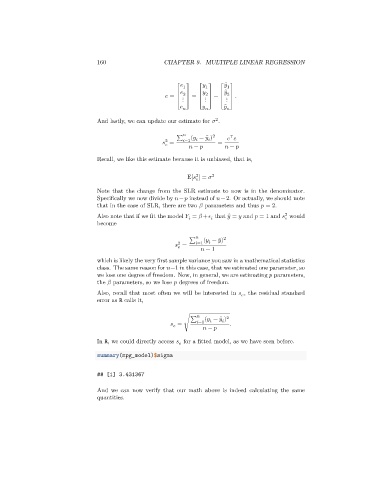
And lastly, we can update our estimate for .

∑ ( − ̂ ) 2
⊤

2
= =1 − = −

Recall, we like this estimate because it is unbiased, that is,
2
E[ ] = 2

Note that the change from the SLR estimate to now is in the denominator.
Specifically we now divide by − instead of −2. Or actually, we should note
that in the case of SLR, there are two parameters and thus = 2.
2

Also note that if we fit the model = + that ̂ = ̄ and = 1 and would

become

∑ ( − ̄) 2

2
= =1

− 1
which is likely the very first sample variance you saw in a mathematical statistics
class. The same reason for −1 in this case, that we estimated one parameter, so
we lose one degree of freedom. Now, in general, we are estimating parameters,
the parameters, so we lose degrees of freedom.
Also, recall that most often we will be interested in , the residual standard

error as R calls it,

∑ ( − ̂ ) 2

= √ =1 − .

In R, we could directly access for a fitted model, as we have seen before.

summary(mpg_model)$sigma

## [1] 3.431367

And we can now verify that our math above is indeed calculating the same
quantities.